The repressilator
(EXAMPLE CONTENT FROM COURSE. LINKS TO OTHER SECTIONS REMOVED)
This lesson will
- introduce you to the concept of systems of differential equations and how they can be solved numerically in MATLAB.
- demonstrate how oscillations can arise in non linear dynamical systems through limit cycles.
The repressilator was a synthetic gene-regulatory network constructed in
Escherichia coli
‡Elowitz:2000gg. Under certain circumstances the network exhibited sustained oscillations as reported through oscillations in Green Fluorescent Protein (GFP). We shall see through analysis of a simple mathemtical model of the network that the sustained oscillations are due to the emergenceEmergence is a key property of systems.
of a limit cycle, a purely non-linear phenomena and extremely important in the modelling of biological processes.
This lesson covers all areas of sections 2.3.2-2.3.5. In addition it also introduces oscillations, the maths of which is covered in section 2.4.
The gene regulatory network
Figure 1.9.1 shows the design of the repressilator and reporter. The main network consists of three genes, each one coding for a protein that acts as a repressing transcription factor for one of the the other genes. This mutually repressing network forms what is called anegative feed back loop
which is shown diagramatically in Figure 1.9.1. The reporter plasmid contained the reporter gene coding for GFP under transcriptional control of the TetR protein causing TetR to repress the production of GFP. Hence the levels of TetR control the levels of GFP in bacteria carrying the two plasmids.
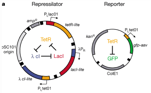
Repressilator design. The three genes code for proteins that repress transcription of exactly one of the other genes. The presence of two difference selection markers,
$amp^R$
and $kan^R$
, ensure that only bacteria carrying both plasmids are present in the experiment. Reprinted by permission from Macmillan Publishers Ltd:
Nature
403
335-338 copyright 2000 The mathematical model
The repressilator network can be modelled via a system of ordinary differential equations. The system is composed of three genes, each coding for an mRNA transcript and the corresponding translated protein. This gives us six species to model and we denote the three mRNA species$m_1, m_2, m_3$
and the three protein species $p_1, p_2, p_3$
where 1,2 and 3 refer to the TetR, $\lambda$
cI and LacI genes respectively. We have a differential equation for the time evolution of each species and the model takes the form
\begin{align}
\frac{ dm_1 }{dt} = -m_1 + \frac{\alpha}{1 + p_3^n } + \alpha_0
&\frac{ dp_1 }{dt} = -\beta (p_1 - m_1) \notag \\
\frac{ dm_2 }{dt} = -m_2 + \frac{\alpha}{1 + p_1^n } + \alpha_0
&\frac{ dp_2 }{dt} = -\beta (p_2 - m_2) \notag \\ \tag{1.9.1}
\frac{ dm_3 }{dt} = -m_3 + \frac{\alpha}{1 + p_2^n } + \alpha_0
&\frac{ dp_3 }{dt} = -\beta (p_3 - m_3),
\label{eqn:repr}
\\ \end{align}
where $\alpha_0$
is the basal rate of expression of each gene, $\alpha$
is the repression strength, $\beta$
is the protein and mRNA degradation rate constant (assumed equal) and $n$
is the Hill coefficient due to the cooperativity of the repression.
Steady state and oscillatory solutions
To numerically integrate the model for the repressilator we need to define the function representing the system of ordinary differential equations. The following function does this, you will need to place it into a file namedrepressilator.m
function ydot=repressilator(t,y,p)
    alpha0 = 1;
    n = 2.0;
    beta = 5;
    alpha = 1000;
    % order of species; y = [m1 p1 m2 p2 m3 p3]
    m1 = -y(1) + alpha/(1+y(6)^n) + alpha0;
    p1 = -beta*(y(2) - y(1));
    m2 = -y(3) + alpha/(1+y(2)^n) + alpha0;
    p2 = -beta*(y(4) - y(3));
    m3 = -y(5) + alpha/(1+y(4)^n) + alpha0;
    p3 = -beta*(y(6) - y(5));
ydot = [m1; p1; m2; p2; m3; p3];$\alpha_0 = 1$
, $n=1$
, $\beta = 5$
and $\alpha = 1000$
. Later on you will see how to make the function accept the parameter values as well.Now we are going to examine the solution to the system when the intial conditions are given by
$m_1,p_1,m_2,p_2,m_3,p_3 =$
$0, 1, 0, 1, 0, 1$
respectively. The following code makes both a time series and a phase space plot for the time interval, $t=[0 \; 15]$
and the results are shown in Figure 1.9.2.timespan=[0 15];
y0 = [0 1 0 1 0 1];
[t,y] = ode45(@repressilator,timespan,y0);
figure()
plot(t,y)
xlabel('Time')
ylabel('Amount')
legend('m1','p1','m2','p2','m3','p3','Location','SouthEast')
figure()
plot(y(:,1), y(:,2))
xlabel('Amount m1')
ylabel('Amount p1')y
from the ode45
function is a matrix. To see that it is a matrixMatrices will be covered in the next submodule.
you can do size(y)
and you will see that it has size $141 \times 6$
which corresponds to 141 rows of six variables; the rows correspond to the time points and the six variables are the concentrations of our species. In the second plot
command we extract column 1 and column 2 from the matrix y
using the syntax y(:,1)
and y(:,2)
. The :
here means "select all" so we are effectively selecting a column. 
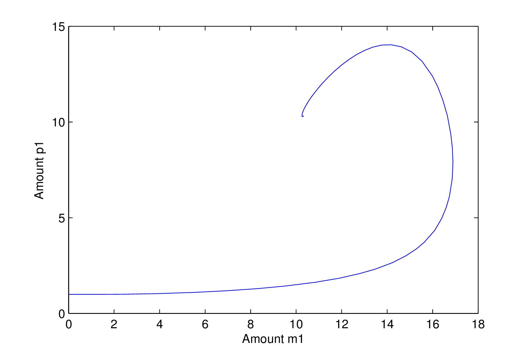
Repressilator with a stable steady state solution
It is clear from the time series in Figure 1.9.2 that the system with these intial conditions eventually ends up at a steady state with all six species taking the same value. The phase space plot shows the trajectory of the two components of the system
$m_1$
and $p_1$
in phase space. The system starts off on the left hand side at the point $m_1=1,p_1=1$
and moves off towards the steady state. Note that the trajectory is not straight and curves, or spirals around the steady state. This type of steady state is known as a stable spiral
. The results woudl be the same for the pairs $m_2, p_2$
and $m_3, p_3$
.- With the same inital contitions $p_1=p_2=p_3=1$,$m_1=m_2=m_3=0$investigate the effect of changing parameter$a$.
- How does this effect the steady state solution?
As we increase and decrease$\alpha$, we see the steady-state solution increases and decreases, respectively. Similarly, the spiral of$m_1$and$p_1$amounts tightens and unravels, respectively.
We shall now see that the repressilator can give sustained oscillations for the same parameters (
$\alpha_0, m, \beta, \alpha$
) but different initial conditions. The following code makes the same plots but for the initial conditions $m_1,p_1,m_2,p_2,m_3,p_3 =$
$0, 1, 0, 2, 0, 5$
. The plots are shown in Figure 1.9.3.
timespan=[0 15];
y0 = [0 1 0 2 0 5];
[t,y] = ode45(@repressilator,timespan,y0);
figure();
plot(t,y)
xlabel('Time')
ylabel('Amount')
legend('m1','p1','m2','p2','m3','p3','Location','NorthWest')
figure();
plot(y(:,1), y(:,2))
xlabel('Amount m1')
ylabel('Amount p1')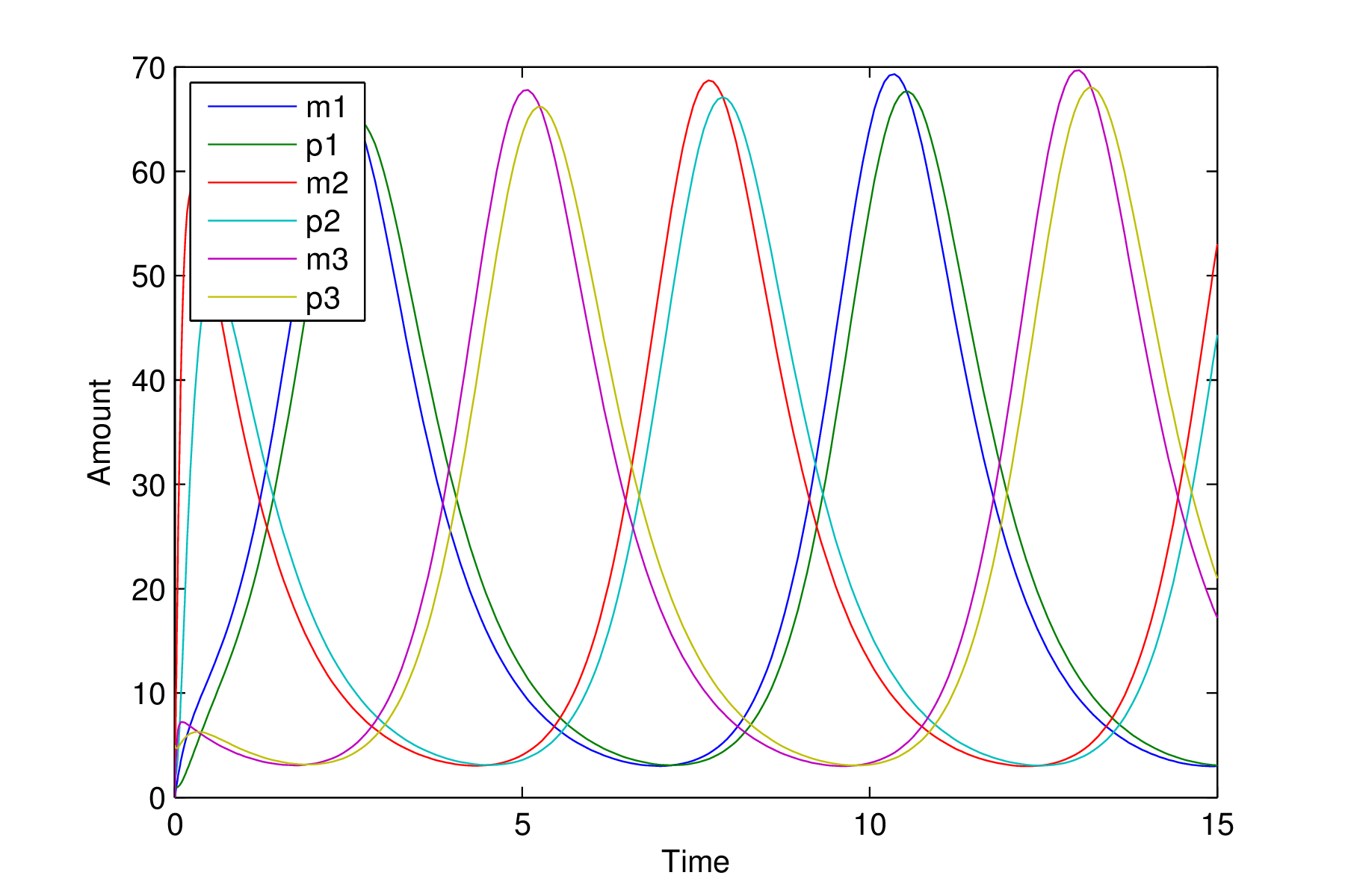
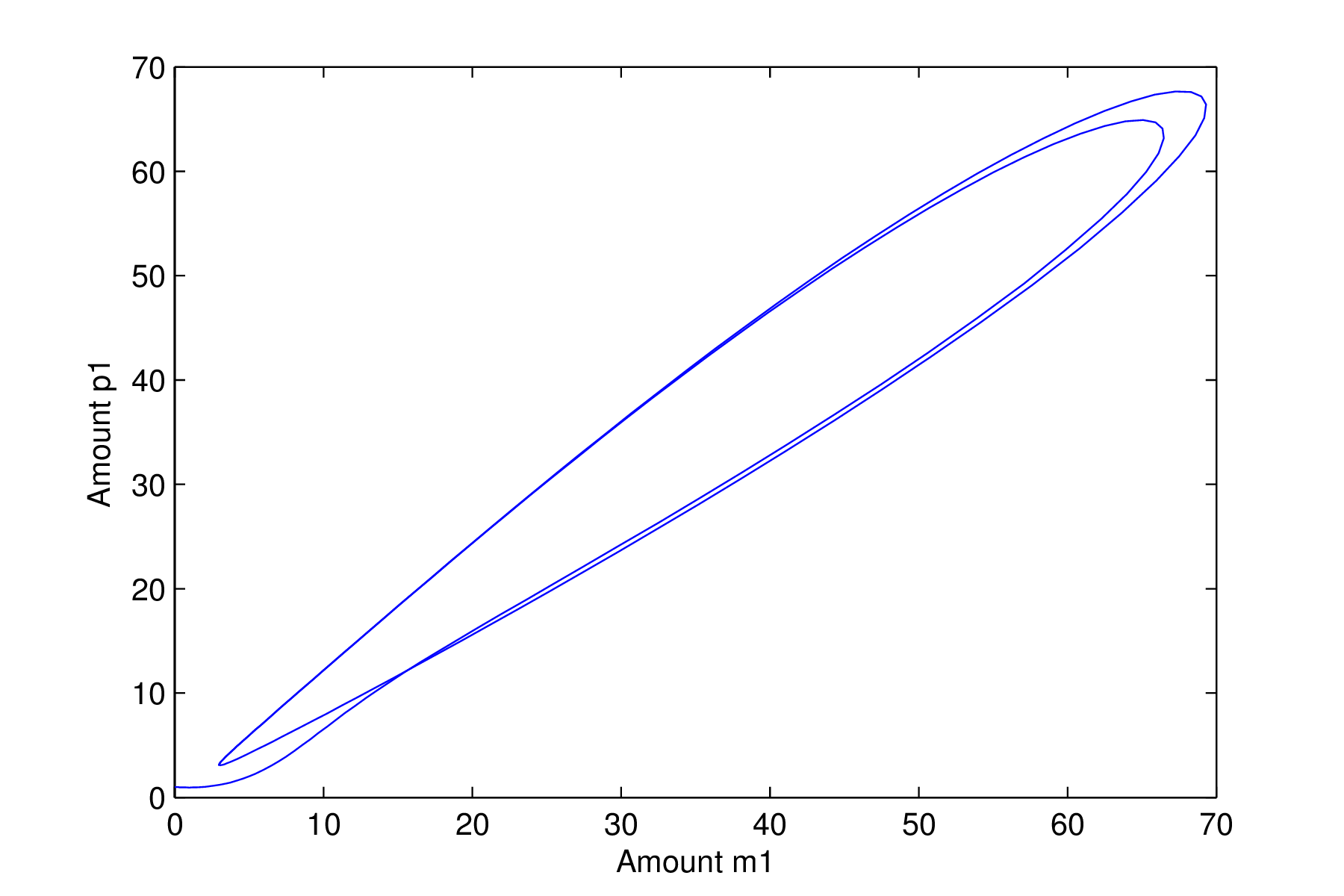
Repressilator with an oscillatory solution
We now see very different behaviour in the system. The time series clearly shows oscillatory solutions and the phase space plot shows the solution moving from the point
$m_1=1,p_1=1$
and quickly moving on to the circular structure where it remains cycling forever. This is known as a limit cycle
We shall examine limit cycles in more detail in
and is the signature of sustained oscillations. This example also demonstrates the concept of "basins of attraction"; depending on where we start the system we may end up with very different behaviour.Module 2
Bifurcations: sudden change in system behaviour
In the previous subsection we saw how the long term system behaviour changed from a stable steady state to a limit cycle and oscillations upon changing the initial conditions. We can also observe this type of transition for fixed initial conditions and changing parameters. This type of behaviour is known as abifurcation
We shall examine bifurcations in more detail in
.Module 2
In order to investigate the system as we change the repression strength,
$\alpha$
, we shall modify our repressilator function so that we can specify the parameters in the argument (rather than hard-coded) and save the file as repressilator2.m
.
function ydot=repressilator2(t,y,p)
    alpha0 = p(1);
    n = p(2);
    beta = p(3);
    alpha = p(4);
    % order of species; y = [m1 p1 m2 p2 m3 p3]
    m1 = -y(1) + alpha/(1+y(6)^n) + alpha0;
    p1 = -beta*(y(2) - y(1));
    m2 = -y(3) + alpha/(1+y(2)^n) + alpha0;
    p2 = -beta*(y(4) - y(3));
    m3 = -y(5) + alpha/(1+y(4)^n) + alpha0;
    p3 = -beta*(y(6) - y(5));
    ydot = [m1; p1; m2; p2; m3; p3];
Now we shall make time series and phase space plots plot for
$\alpha=5,28,1000$
and keeping the rest of the parameters fixed.
timespan=[0 15];
y0 = [0 1 0 2 0 3];
params1 = [1 1.75 5 5];
params2 = [1 1.75 5 28];
params3 = [1 1.75 5 1000];
[t1,y1] = ode45(@repressilator2,timespan,y0,[],params1);
[t2,y2] = ode45(@repressilator2,timespan,y0,[],params2);
[t3,y3] = ode45(@repressilator2,timespan,y0,[],params3);
figure();
subplot(3,1,1)
plot(t1,y1)
ylabel('Amount')
subplot(3,1,2)
plot(t2,y2)
ylabel('Amount')
subplot(3,1,3)
plot(t3,y3)
xlabel('Time')
ylabel('Amount')
figure();
subplot(3,1,1)
plot(y1(:,1), y1(:,2))
ylabel('Amount p1')
subplot(3,1,2)
plot(y2(:,1), y2(:,2))
ylabel('Amount p1')
subplot(3,1,3)
plot(y3(:,1), y3(:,2))
xlabel('Amount m1')
ylabel('Amount p1')ode45
you will see that the third argument must be a structure and we do not want to use this so we pass an empty array.The resulant plots are shown in Figures 1.9.4 and 1.9.5.
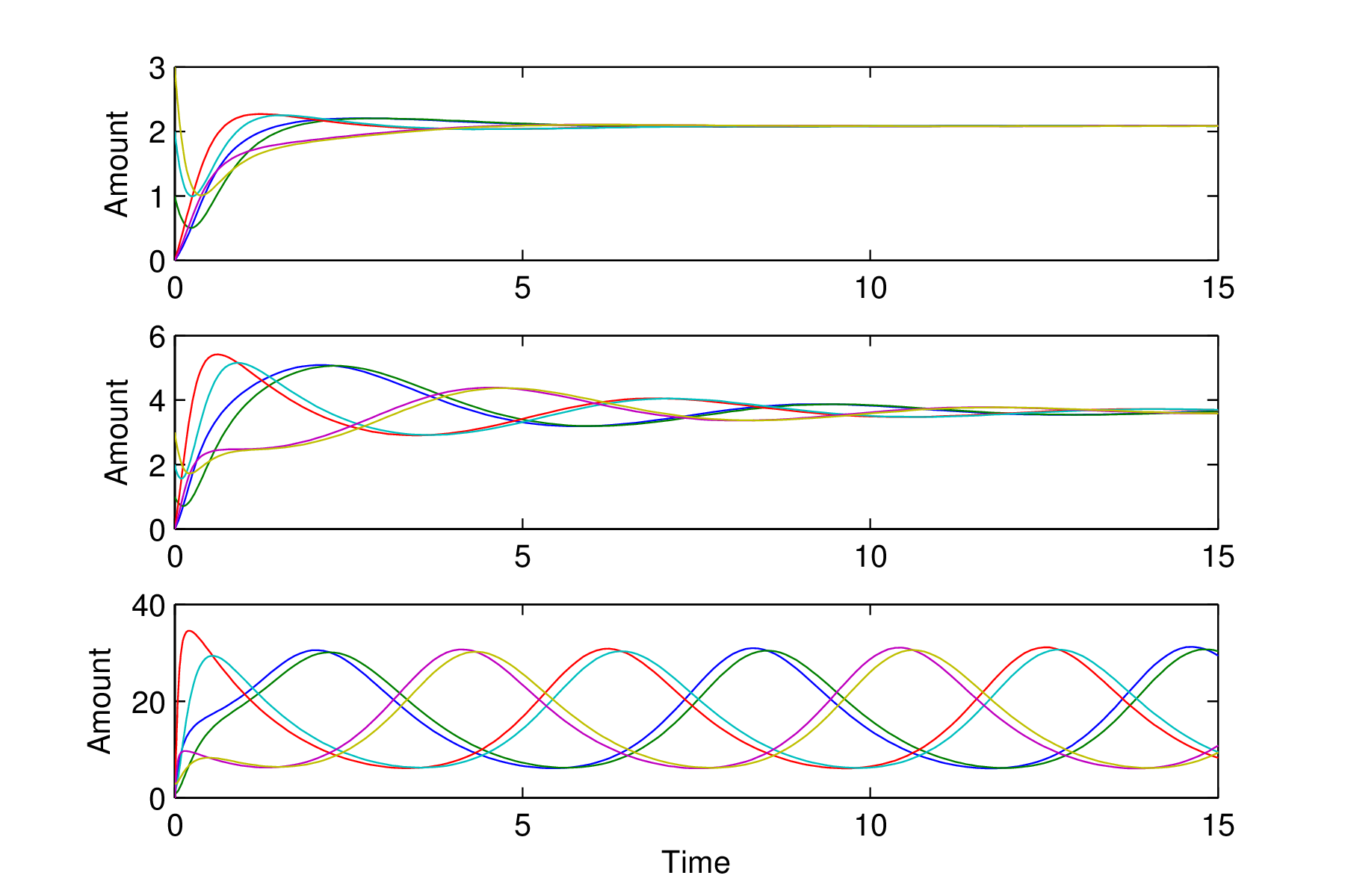
The changing behaviour of the repressilator solutions

The phase space of the repressilator undergoing a Hopf bifurcation
Figures 1.9.4 and 1.9.5 clearly show the system moving from steady state behaviour through damped oscillations to sustained oscillations. This type of behaviour is known as a
Hopf bifurcation
. What happens is that the steady state is stable but the trajectories become more strongly spiral in nature which gives rise to the damped oscillations. Suddenly at a particular value of $\alpha$
(here between 28 and 29) the steady state becomes unstable and a limit cycle suddenly emerges. All trajectories move onto the limit cycle and remain there giving sustained oscillations- A modification of the repressilator is to use a cyclic network of four genes, where each gene codes the repressing transcription factor for the next gene in the cycle.
Modify the MATLAB repressilator function to make this network setting$\alpha_0 = 1$,$n=1$,$\beta = 5$and$\alpha = 1000$. - Experiment with adjusting initial concentrations. You should be able to make the circuit produce two different final states (e.g. you might find differentsteady states and/or show oscillations). Plot the graphs of the solutions you found.
- Try a few different sets of parameters. Do any of them produce limit cycle (sustained) oscillations?
- Optional extension work: Consider the differences between the three and four gene networks. Can you reason why they have different behaviours? What would happen with a five gene network? Has anyone done this experimentally?